
Did our posner experiment work? lets look at plotting the data from a single participant
There are many different libraries for data analysis in Python. But today we will mention just a few:
numpy : Fast multi-dimensional arrays, basic numeric operations
pandas : Very similar to numpy but supporting named columns
matplotlib : Visualization
scipy : Many basic scientific functions (including inferential stats)
A more detailed version of these slides can be found at
This library is at the peak of the ecosystem. Everything depends on this. It includes an implementation of multi-dimensional arrays with different data-types.
This is a very simple concept, but also a very powerful one!
It also contains some basic mathematical functions to operate on these arrays
To create an array, you may pass a sequence of elements into the numpy.array function:
import numpy as np
my_array = np.array([1,2,3])
This object has a shape attribute, that reports on its size:
print(my_array.shape)
And a dtype attribute, that reports on its data-type:
print(my_array.dtype)
This doesn’t seem very interesting, but consider a slightly more complicated array:
my_array = np.array([[1, 2, 3], [4, 5, 6]])
print(my_array.shape)
A 2d array can be considered a matrix.
You can automatically create an array with a range of numbers:
first_way = np.arange(0, 10.5, 0.5)
another_way = np.linspace(0, 10, 21)
print(first_way)
print(another_way)
And you can determine the shape you want it to have:
ten_by_ten = np.arange(100).reshape((10, 10))
print(ten_by_ten)
Exercise: Using numpy 1. make a list ranging 0 to 1 with 90 steps 2. print the shape of the array 3. reshape the array to be 3 rows of 30 4. print only the final row from the matrix
There are many functions in the numpy name-space to do operations on arrays:
print(np.mean(ten_by_ten))
print(np.mean(ten_by_ten, axis=0))
print(np.sqrt(ten_by_ten))
Matplotlib is very general and customizable. There are several different interfaces to the objects and functions implemented in MPL:
matplotlib - raw access to the plotting library. useful for extending matplotlib or doing very custom things
pylab - Matlab-like interface to matplotlib
pyplot - Object-oriented interface to matplotlib => use this one!
To create a figure and start plotting data:
import matplotlib.pyplot as plt
fig, ax = plt.subplots(1)
The two objects returned from this call are a matplotlib.figure.Figure
and matplotlib.axes.AxesSubplot. They each have multiple methods that
can now be used.
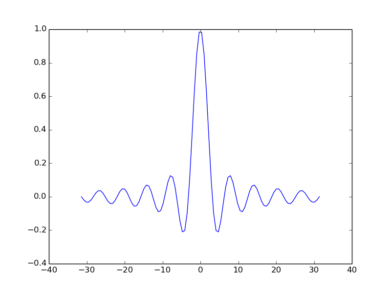
For example:
t = np.linspace(-6*np.pi, 6*np.pi, 100)
ax.plot(t, np.sin(t)/t)
plt.show()
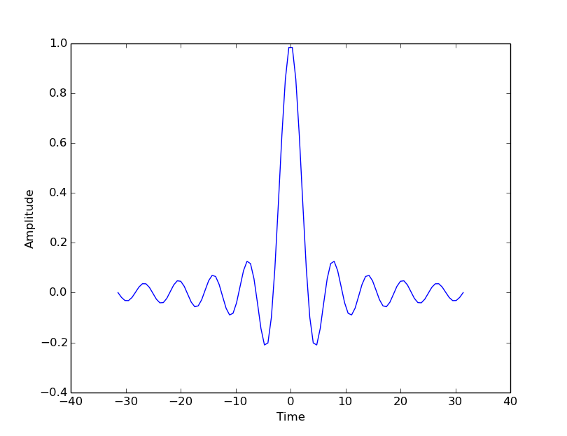
Use the object’s ‘setter’ functions, to set various attrbutes of the arrays. For example:
ax.set_xlabel('Time')
ax.set_ylabel('Amplitude')
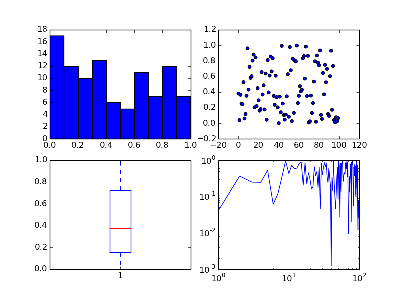
The subplots command can return an array of axes:
fig, ax = plt.subplots(2,2)
We can plot different kinds of plots in each one:
x = np.arange(0, 100)
y = np.random.rand(100)  # 100 random numbers
ax[0, 0].hist(y)
ax[0, 1].scatter(x, y)
ax[1, 0].boxplot(y)
ax[1, 1].loglog(x, y)
To show both figures call plt.show() at the end of the script.
Take a look at the Matplotlib gallery for many examples.
Each thumb-nail in the gallery contains a link to a page that has the source code that created that image. Use the code as a starting point for your own visualization.
There are two simple ways to find files. You could search for all files in a folder using a module called glob:
import glob
filenames = glob.glob("data/*.csv")
Or you could open a file dialog using PsychoPy:
from psychopy import gui
filenames = gui.fileOpenDlg(allowed="*.csv")
Either way you get a list of file paths a list (which might be empty).
It’s also useful to have something to manipulate filenames. We’ll use os.path for that:
from os import path
from psychopy import gui
filenames = gui.fileOpenDlg(allowed="*.csv")
for thisFilename in filenames:
    thisPath, thisFullName = path.split(thisFilename)
    fileNoExt, fileExt = path.splitext(thisFilename)
    print('thisPath:', thisPath, 'thisFullName:', thisFullName)
    print('this fileNoExt:', fileNoExt, 'this fileExt:', fileExt)
Use a similar trick to the last one but we’re going to use another library called pandas (http://pandas.pydata.org/)
from os import path
from psychopy import misc, gui
import pandas as pd

filenames = gui.fileOpenDlg(allowed="*.csv")
for thisFilename in filenames:
    print(thisFilename)
    thisDat = pd.read_csv(thisFilename)
    print(thisDat)
Boom! We’ve got our data, as easily as that!
But, really, how easily can we use that data? Let’s try to pull out just the reaction times:
for thisFilename in filenames:
    print(thisFilename)
    thisDat = pd.read_csv(thisFilename)
    print(thisDat['rt'])
We can also select parts of the data that fulfill certain criteria. Let’s get rid of trials where rt>1.0 (not ready?) and corr==0:
for thisFilename in filenames:
    print(thisFilename)
    thisDat = pd.read_csv(thisFilename)
    #filter out bad data
    filtered = thisDat[ thisDat['rt']<=1.0 ]
    filtered = filtered[ filtered['corr']==1 ]
    print(filtered['rt'])
OK, from our filtered data we need the mean and std.dev. reaction time for each condition:
import scipy
from scipy import stats
...

conflict = filtered[filtered.descr == 'conflict']
congruent = filtered[filtered.descr != 'conflict']
#get mean/std.dev
meanConfl = scipy.mean(conflict['rt'])
sdConfl = scipy.std(conflict['rt'], ddof=1) # ddof=1 means /sqrt(N-1)
meanCongr = scipy.mean(congruent['rt'])
sdCongr = scipy.std(congruent['rt'], ddof=1)
print("Conflict = %.3f (sd=%.3f)" %(meanConfl, sdConfl))
print("Congruent = %.3f (sd=%.3f)" %(meanCongr, sdCongr))
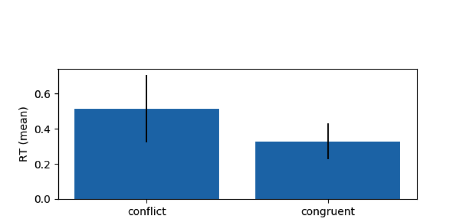
Let’s plot our data from the posner experiment:
    import matplotlib.pyplot as plt
fig, ax = plt.subplots(1)
ax.bar(['Conflict', 'Congruent'], [meanConfl, meanCongr], yerr=[sdConfl, sdCongr])
ax.set_ylabel('RT (mean)')
plt.show()
If you want to save the Figure:
fig.savefig('my_figure.png')
fig.savefig('my_figure.pdf')
Exercise Create a three panel figure, something like this:
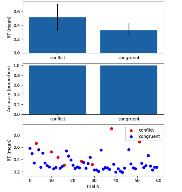
Solution:
fig, ax = plt.subplots(3)
ax[0].bar(['conflict', 'congruent'], [meanConfl, meanCongr], yerr=[sdConfl, sdCongr])
ax[0].set_ylabel('RT (mean)')

ax[1].bar(['conflict', 'congruent'], [AccConfl, AccCongr])
ax[1].set_ylabel('Accuracy (proportion)')

ax[2].scatter(conflict['MainBlock.thisN'], conflict['rt'],
c = 'r', label = 'conflict')
ax[2].scatter(congruent['MainBlock.thisN'], congruent['rt'],
c = 'b', label = 'congruent')
ax[2].set_ylabel('RT (mean)')
ax[2].set_xlabel('trial N')
ax[2].legend(loc = 'upper right')
Exercise Now collect another set of posner data, and try to plot for each participant in turn
This contains an implementation of many of the core computational routines you need in scientific computing:
scipy.cluster : Vector quantization / Kmeans
scipy.constants : Physical and mathematical constants
scipy.fftpack : Fourier transform
scipy.integrate : Integration routines
scipy.interpolate : Interpolation
scipy.io : Data input and output
scipy.linalg : Linear algebra routines
scipy.ndimage : n-dimensional image package
scipy.odr : Orthogonal distance regression
scipy.optimize : Optimization
scipy.signal : Signal processing
scipy.sparse : Sparse matrices
scipy.spatial : Spatial data structures and algorithms
scipy.special : Any special mathematical functions
scipy.stats : Statistics
Is the difference in RT between congruent and conflict responses significant (at the group level)?
Make sure you have multiple files to select and before your loop create an empty list where you will store each participants mean RT:
Confl_mean_rts=[]
Congr_mean_rts=[]
Then, once you have calculated each participants mean, append the list:
#in your loop
Confl_mean_rts.append(meanConfl)
Congr_mean_rts.append(meanCongr)
Finally, test congruent and incongruent RTs using a paired samples t-test:
t, p = stats.ttest_rel(Confl_mean_rts, Congr_mean_rts)
print("Related samples t-test: t=%.3f, p=%.4f"%(t, p))
Note we must have even observations (and more than one observation) for this to run.
Realistically, we would rarely perform inferential statistics at the single subject level. At the group level, we would have one value per condition per participant (so even observations).
Hopefully today you have learnt how to:
Create an experiment using only python code in PsychoPy
Optimise the experiment
Visualise the results (and move forward with analysing them)
What else? Python syntax and objects