
In most cases you don’t need to be able to program to analyse the data. You could do all your analyses in Excel and SPSS.
On the other hand, a Python script might be useful in performing repeated analyses. Do you never tweak and re-run an analysis?
There are many different libraries for data analysis in Python. This forms an expansive eco-system of different functionalities. Google “XXX python” and someone is likely to have implemented it.
We will discuss four of the core libraries on which all the rest rely:
numpy : Fast multi-dimensional arrays, basic numeric operations
pandas : Very similar to numpy but supporting named columns
scipy : Many basic scientific functions
matplotlib : Visualization
ipython : interactive analysis
This library is at the peak of the ecosystem. Everything depends on this. It includes an implementation of multi-dimensional arrays with different data-types.
This is a very simple concept, but also a very powerful one!
It also contains some basic mathematical functions to operate on these arrays
To create an array, you may pass a sequence of elements into the numpy.array function:
import numpy as np
my_array = np.array([1,2,3])
This object has a shape attribute, that reports on its size:
print(my_array.shape)
And a dtype attribute, that reports on its data-type:
print(my_array.dtype)
This doesn’t seem very interesting, but consider a slightly more complicated array:
my_array = np.array([[1, 2, 3], [4, 5, 6]])
print(my_array.shape)
You can automatically create an array with a range of numbers:
first_way = np.arange(0, 10.5, 0.5)
another_way = np.linspace(0, 10, 21)
print(first_way)
print(another_way)
And you can determine the shape you want it to have:
ten_by_ten = np.arange(100).reshape((10, 10))
print(ten_by_ten)
Arrays can be used to do math. Let’s demonstrate with a simple array containing integer values:
a = np.array([[1, 2, 3,], [4, 5, 6]])
print(a.shape)
(2, 3)
Math between an array and a scalar applies the computation between the scalar and each element of the array:
a2 = a + 2
print(a2)
array([[3, 4, 5], [6, 7, 8]])
Exercise: If you have an array that contains image values, how would you double its contrast?
Math between arrays proceeds element-by-element.
Therefore, it can only be done for arrays with the same shape:
b = np.array([[6, 5, 4], [3, 2, 1]])
c = a + b
print(c)
[[7 7 7]
 [7 7 7]]
This can be done with other binary operators as well:
d = a ** b
print(d)
[[ 1 32 81]
[64 25  6]]
There are many functions in the numpy name-space to do operations on arrays:
print(np.mean(d))
print(np.mean(d, axis=0))
print(np.sqrt(d))
Arrays can be treated as 2-dimensional matrices and we can do matrix operations between them.
Note
We’ve already seen that for addition, because matrix addition is simply element-by-element addition. What about matrix multiplication?
There are a couple of different ways to do this, but the simplest is using the numpy.dot function. This works for linear (1D) arrays:
a = np.array([1, 2, 3, 4, 5, 6, 7])
b = np.array([7, 6, 5, 4, 3, 2, 1])
c = np.dot(a,b)
As well as for multi-dimensional arrays:
a = np.array([[1, 2, 3, 4], [5, 6, 7, 8]])
b = np.array([[1, 2], [3, 4], [5, 6], [7, 8]])
c = np.dot(a, b)
Can you multiply np.dot(b, a)?
How about if this was the case?:
b = np.array([[1, 2], [3, 4], [5, 6]])
What happens when the array has more than 2 dimensions?
A few useful kinds of arrays:
ones33 = np.ones([3, 3])
zeros33 = np.zeros([3, 3])
eye33 = np.eye(3)
empty33 = np.empty([3, 3])
Why would you need an empty array?
Logical operations with arrays produces arrays of boolean dtype:
a = np.array([1, 2, 3, 4, 5, 6, 7])
b = np.array([7, 6, 5, 4, 3, 2, 1])
c = (a==b)
print(c)
This can be used for indexing:
print(a[a==b])
You can’t directly use this as a test though. Try:
if a==b:
   print("a is equal to b")
Why do you think that doesn’t work?
Instead, you can use np.all or np.any:
print(np.any(a==b))
print(np.all(a==b))
print(np.all(a==a))
print(np.any(a==a))
This contains an implementation of many of the core computational routines you need in scientific computing:
scipy.cluster : Vector quantization / Kmeans
scipy.constants : Physical and mathematical constants
scipy.fftpack : Fourier transform
scipy.integrate : Integration routines
scipy.interpolate : Interpolation
scipy.io : Data input and output
scipy.linalg : Linear algebra routines
scipy.ndimage : n-dimensional image package
scipy.odr : Orthogonal distance regression
scipy.optimize : Optimization
scipy.signal : Signal processing
scipy.sparse : Sparse matrices
scipy.spatial : Spatial data structures and algorithms
scipy.special : Any special mathematical functions
scipy.stats : Statistics
import scipy.fftpack as fft
my_ft = fft.fft(np.random.randn(2,100))
print(my_ft)
Lot’s of useful examples and study materials to be found here
Matplotlib is very general and customizable. For most usages, you don’t actually need to interact with all that power. There are several different interfaces to the objects and functions implemented in MPL:
- matplotlib - raw access to the plotting library. useful for extending
matplotlib or doing very custom things
pylab - Matlab-like interface to matplotlib
pyplot - Object-oriented interface to matplotlib => use this one!
To create a figure and start plotting data:
import matplotlib.pyplot as plt
fig, ax = plt.subplots(1)
The two objects returned from this call are a matplotlib.figure.Figure
and matplotlib.axes.AxesSubplot. They each have multiple methods that
can now be used.
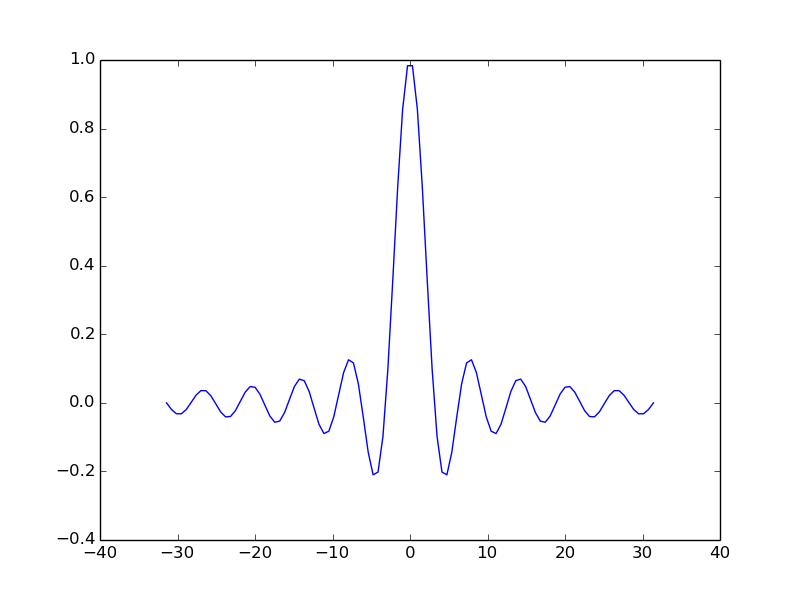
For example:
t = np.linspace(-6*np.pi, 6*np.pi, 100)
ax.plot(t, np.sin(t)/t)
plt.show()
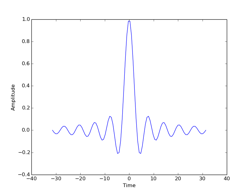
Use the object’s ‘setter’ functions, to set various attrbutes of the arrays. For example:
ax.set_xlabel('Time')
ax.set_ylabel('Amplitude')
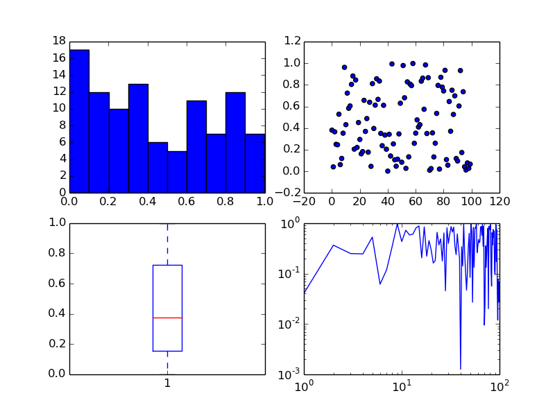
The subplots command can return an array of axes:
fig, ax = plt.subplots(2,2)
We can plot different kinds of plots in each one:
x = np.arange(0, 100)
y = np.random.rand(100)  # 100 random numbers
ax[0, 0].hist(y)
ax[0, 1].scatter(x, y)
ax[1, 0].boxplot(y)
ax[1, 1].loglog(x, y)
We can read images from files into arrays:
img1 = plt.imread('images/lena.png')
Or generate our own 2D arrays:
img2 = np.random.rand(128, 128)
fig, (ax1, ax2) = plt.subplots(1, 2)
ax1.imshow(img1)
ax2.imshow(img2)
ax1.set_axis_off()  # Hide "spines" on first axis
Take a look at the Matplotlib gallery for many examples.
Each thumb-nail in the gallery contains a link to a page that has the source code that created that image. Use the code as a starting point for your own visualization.
The basic functionality of ipython is a more pleasant python interperter that runs in the terminal. It has many things that make life easier
But there are a few other features:
Interactive shells (terminal Qt-based).
Interactive notebook.
Interactive data visualization.
Parallel computing.
There are a couple of easy ways to install all of these things together on any platform:
They both contain package managers, which will help you install other libraries. They’re both free for academic use.
Various options:
csv file for the experiment (one trial per line)
csv or excel ‘summaries’ format (can only be saved by individual loops, not the ExperimentHandler). Not really recommended any more.
log files (not for analysis though)
- psydat files (literally a saved copy of the Experiment/TrialHandler)
can save fresh copies of the csv file from here too
in future should be able to export a copy of the original script that collected the data as well
There are two simple ways to find files. You could search for all files in a folder using a module called glob:
import glob
filenames = glob.glob("data/*.csv")
Or you could open a file dialog using PsychoPy:
from psychopy import gui
filenames = gui.fileOpenDlg(allowed="*.csv")
Either way you get a list of file paths a list (which might be empty).
It’s also useful to have something to manipulate filenames. We’ll use os.path for that:
from os import path
from psychopy import gui
filenames = gui.fileOpenDlg(allowed="*.csv")
for thisFilename in filenames:
    thisPath, thisFullName = path.split(thisFilename)
    fileNoExt, fileExt = path.splitext(thisFilename)
    print(thisPath, thisFullName)
    print(fileNoExt, fileExt)
Use a similar trick to the last one but we’re going to use another library called pandas (http://pandas.pydata.org/)
from os import path
from psychopy import misc, gui
import pandas as pd

filenames = gui.fileOpenDlg(allowed="*.csv")
for thisFilename in filenames:
    print(thisFilename)
    thisDat = pd.read_csv(thisFilename)
    print(thisDat)
Boom! We’ve got our data, as easily as that!
But, really, how easily can we use that data? Let’s try to pull out just the reaction times:
for thisFilename in filenames:
    print(thisFilename)
    thisDat = pd.read_csv(thisFilename)
    print(thisDat['rt'])
We can also select parts of the data that fulfill certain criteria. Let’s get rid of trials where rt>1.0 (not ready?) and corr==0:
for thisFilename in filenames:
    print(thisFilename)
    thisDat = pd.read_csv(thisFilename)
    #filter out bad data
    filtered = thisDat[ thisDat['rt']<=1.0 ]
    filtered = filtered[ filtered['corr']==1 ]
    print(filtered['rt'])
OK, from our filtered data we need the mean and std.dev. reaction time for each condition:
import scipy
from scipy import stats
...

conflict = filtered[filtered.descr == 'conflict']
congruent = filtered[filtered.descr != 'conflict']
#get mean/std.dev
meanConfl = scipy.mean(conflict['rt'])
sdConfl = scipy.std(conflict['rt'], ddof=1) # ddof=1 means /sqrt(N-1)
meanCongr = scipy.mean(congruent['rt'])
sdCongr = scipy.std(congruent['rt'], ddof=1)
print("Conflict = %.3f (sd=%.3f)" %(meanConfl, sdConfl))
print("Congruent = %.3f (sd=%.3f)" %(meanCongr, sdCongr))
Yes, but, I mean really, is that significant?:
t, p = stats.ttest_ind(conflictRT, congruentRT)
print("Independent samples t-test: t=%.3f, p=%.4f")
(Note that this is doing the statistics for a single participant, not the stats across a group).
You can fetch working copies of those analysis scripts, and data file to test them on from here:
You could open this for analysis, but for now let’s use it to try saving out new copies of data (make sure your undergrads didn’t fudge their results?!)
from psychopy import misc
dat = misc.fromFile( someFileNameHere )
dat.saveAsWideText( newFileNameHere )
OK, let’s open a set of psydat files and output new copies of the csv file:
from os import path
from psychopy import misc, gui
filenames = gui.fileOpenDlg(allowed="*.psydat")
for thisFilename in filenames:
    fileNoExt, fileExt = path.splitext(thisFilename)
    newName = fileNoExt+"NEW.csv"
    dat = misc.fromFile(thisFilename)
    dat.saveAsWideText(newName)
    print('saved', newName)
Let’s apply our knowledge to the data from the posner experiment:
fig, ax = plt.subplots(1)
ax.bar([1,2], [meanConfl, meanCongr], yerr=[sdConfl, sdCongr])
plt.show()
If you want to save the Figure:
fig.savefig('my_figure.png')
fig.savefig('my_figure.pdf')